Herbgrind Part 8: The Local Machine In Practice

Welcome back to my series of posts on Herbgrind, a dynamic analysis tool that finds floating point issues in compiled programs. The purpose of this series is to explain how Herbgrind works and the principles behind its design. To do that, we started with a simple hypothetical computer called the “Float Machine”, which is just enough to capture the interesting floating point behavior of a practical computer, like the one that’s probably sitting on your desk. Now, we’re bringing Herbgrind’s analysis to the real world, making it computable and fast.

If you missed the previous posts in this series, you might find this one a bit confusing, so I suggest you go back and read it from the beginning. If that’s too much reading, the post on building a valgrind tool has a short summary of the lead up, and introduces the Valgrind framework which this post builds on. In this post, I’m going to assume you know what I mean when I talk about “the Local Machine”, or “thread state”.

We’ve already talked a lot about the Real Machine, a machine that executes programs in parallel with their regular execution, but uses Real numbers instead of floating point ones. Thanks to the Real Machine, we can figure out the “correct” answer for a floating point program, and we can compare it to the one that gets computed by the program using floating point. This let’s us tell the user how much error each result had when all is said and done.

But just knowing that error is a problem isn’t enough; we need to enable the user to fix the error. The next machine, the Local Machine, tracks down where the error first appears, so we can go about fixing it. But not all the places where error appears are that bad: sometimes error appears in one place, but doesn’t get big enough to affect anything important, or ends up going nowhere. So the task of the Local Machine is twofold: figure out where error is coming from, and figure out where it goes.

Where Error Comes From

In the post on the Local Machine, we developed the notion of “local error”, the error that a single operation has, independent of any error around it. We found that we can discover the local error of an operation by using exact values for its arguments, from the Real Machine, and then rounding them and executing the operation on floats. The difference between this result and the exact result is the local error of the operation on those inputs.

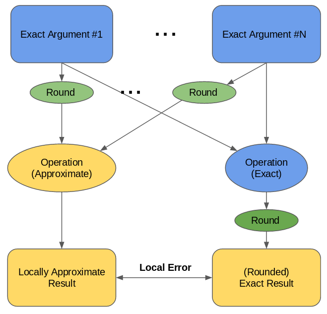
To find local error, two executions on the exact arguments are compared: one which rounds before the computation, and one which rounds after

Doing this in on a practical computer, using the Valgrind framework, is pretty straightforward. We already know from the last post that we have shadow values for each argument, sitting around in memory somewhere. VEX only allows operations to be executed on temporaries (values in memory or thread state have to first be moved to temporaries), so we don’t have to consider the case where the shadow value is in the memory hash table, or thread state shadow storage. When we see an operation whose local error we want to evaluate, we know that the exact values of its arguments are in the shadow temporaries that correspond to its argument temporaries.

MPFR provides an API for taking an exact shadow value, and rounding it to a double- or single- precision float. There’s a lot of flexibility in how you do this (so many rounding modes…), but we just round down all the time.

To compute local error properly, we need to round to the precision of the original operation. Otherwise, if we try to compute the local error of a single-precision operation using a double-precision rounding, we might miss the error entirely, and never detect local error even when global error grows. On the other hand, if we try to compute the local error of a double-precision operation using a single-precision rounding, we’ll detect error that doesn’t really exist. Luckily it’s pretty easy to tell what the precision of the original operation is, just by looking at the instruction it uses: processors tend to have different instructions for dealing with single-precision floats and double-precision floats, and VEX preserves this distinction.

For operations which aren’t a single instruction, but are instead a wrapped library call, we don’t have an instruction code to look at, but instead use the type of the function that was called. In libm (and any implementation of math.h, the standard API for math libraries in C), there are generally two versions of any function, one for double precision (the default, for instance sqrt), and one for single precision (usually with a suffix of f, like sqrtf).

Once we’ve got the exact arguments rounded, we just need to run the “normal” operation on them, and compare the result to the exact answer. When the original operation is something basic like addition, or division, we can do this using the built in operators in C, as long as we make sure to specify the types in the right places. We saw in the last post that because of the way Valgrind interacts with the C standard library, when the original operation is a library call we can’t run the “normal” by just calling the original libm implementation, but luckily we’ve already set up the machinery to call the OpenLibm implementation instead. OpenLibm, as a fully functional implementation of math.h, also includes the single-precision versions of all the functions.

So the steps to computing local error are:

1. Get the argument and result locations of the original operation
2. Grab the shadow arguments from the shadow temporaries corresponding to the original arguments.
3. Round the shadow real value of each argument down to the precision of the original operation.
4. Pass the rounded arguments to the OpenLibm version of the original operation, to get the “locally approximate” result.
5. Grab the shadow result from the shadow temporary corresponding to the original result.
6. Round the shadow real value of the result down to the precision of the original operation.
7. Compare the “exact” result to the “locally approximate” result to get the local error.

Once we can compute the local error for each operation, we can figure out where the error in a program is “coming from”, by just looking for the operations with lots of local error! The local error of different operations doesn’t interact, since we start from exact arguments every time, so we get a good measure of the error that arises from that operation alone.

Where Error Goes

The second job of the local machine is tracking the “influence” of erroneous code on the final results of the program. Without this, we could report all the sources of error to the user, but we wouldn’t know which ones were important, and which ones end up going nowhere.

In the original Local Machine post, for the abstract Float Machine, we talked about tracking these influences through a “taint analysis”; which means we generate a “taint” on some event, and propagate that taint (copy it) from the arguments of certain operations to their results. In the case of our local error analysis, we generate a “taint” every time we see local error above some threshold (5 bits by default¹). And at every operation we shadow, we copy the taints from the arguments to the result.

For the purposes of the local machine, we’ll call our taints “influences”. Each influence is an object that points to a specific operation, where local error occurred. When we first run into local error, we create a new influence which points to the current operation, and we add it to the current shadow value’s influence set. Since each shadow value also holds the influences from the shadow values used to create it, at each operation we have: the influences from the arguments, union-ed together, and an influence for the current operation if it had significant local error.

With this system we can figure out which operations with error influenced each other, but we still have to figure out which values are “outputs”, in that we care about their results for program correctness.

Originally in Herbgrind we asked the user to mark these values explicitly, but that involved a lot of manual labor, and required understanding the program that you wanted to analyze, which we don’t always want to make a requirement. So instead, we now automatically infer the outputs of the program based on a couple of conditions.

The intuition behind this system is that you only care about floating point values you can “see”; out of sight, out of mind. While you’re doing operations on floating point values, they are just bits in memory, so it doesn’t yet matter how accurate they are. It’s only when you use them to change observable behavior that you care about their accuracy. There are a few ways you can “observe” floating point values: you can print them to the screen, you can compare them to another value to make some sort of decision in the program, or you can convert them to an integer. The last one might seem a little weird, since integers are still just bits in memory, and aren’t necessarily directly observable, but any integer might become observable later, and so to avoid having to track integer values, we just flag floating point values on a conversion to int as well. Luckily these conversions are infrequent enough to avoid overwhelming the user with “fake” outputs.

Detecting each of these “observation” events involves a slightly different mechanism. For the first event, printing of floats, we do a similar trick as with math wrapping from the previous post, but instead of wrapping functions like sqrt, we wrap the printing functions like printf². To detect comparisons, we just look for instances of the VEX compare instructions, and to detect conversions to integers we look for the VEX instructions which convert floating-point values to integers.

Putting it All Together

To give the user the most complete picture of the error’s impact, we want to tell them, for each observation:

1. How often it happened
2. Which operations with high local error flowed into it
3. How accurate the result of the observation was, both on average and in the worst case

Counting how often each observation point is hit is pretty easy: we just have an integer counter in its record, and increment it every time we hit the observation. Keeping track of the influences is slightly more complicated, but we’ve outlined above how that happens. Tracking the accuracy, though, gets a little tricky.

What does it mean for an observation to be accurate? Well, for different observations, it means different things. For print observations, since we might be printing out an arbitrary amount of the floating point value, we’ll use our general metrics for floating point accuracy: how many bits of the result are correct. For integer conversions and floating point comparisons, we’ll do something a little more course grained, and just measure accuracy as either “right” or “wrong”. If a comparison returns the same value for both the computed and shadow values, it’s “right”; otherwise it’s “wrong”. Likewise, if a conversion produces the same integer for both the computed and shadow values, it’s “right”; otherwise it’s “wrong”.

That’s pretty much it for local error! I think the transformation from the abstract Local Machine to an actual implementation is simpler than some of the other implementations; so much of the complexity is captured in the abstract model.

For a final closing blurb, I recently designed a new “drawing” version of the Herbgrind logo, a little more cleaned up than the photo version, for using on slides and such. Here’s its official debut:

See you next time!