Herbgrind Part 3: The Localizing Machine

Welcome back to my series of posts on Herbgrind, a dynamic analysis tool that finds floating point issues in compiled programs. The purpose of this series is to explain how Herbgrind works and the principles behind its design. To do that, we’re starting with a simple hypothetical computer called the “Float Machine”, which is just enough to capture the interesting floating point behavior of a real computer, like the one that’s probably sitting on your desk.

In the previous post, we added a machine to Herbgrind that could evaluate the accuracy (or lack thereof) of the final result of a program. But knowing how inaccrate your program is is only part of the solution. To actually repair the program, you need to know where the inaccuracy comes from, and why.

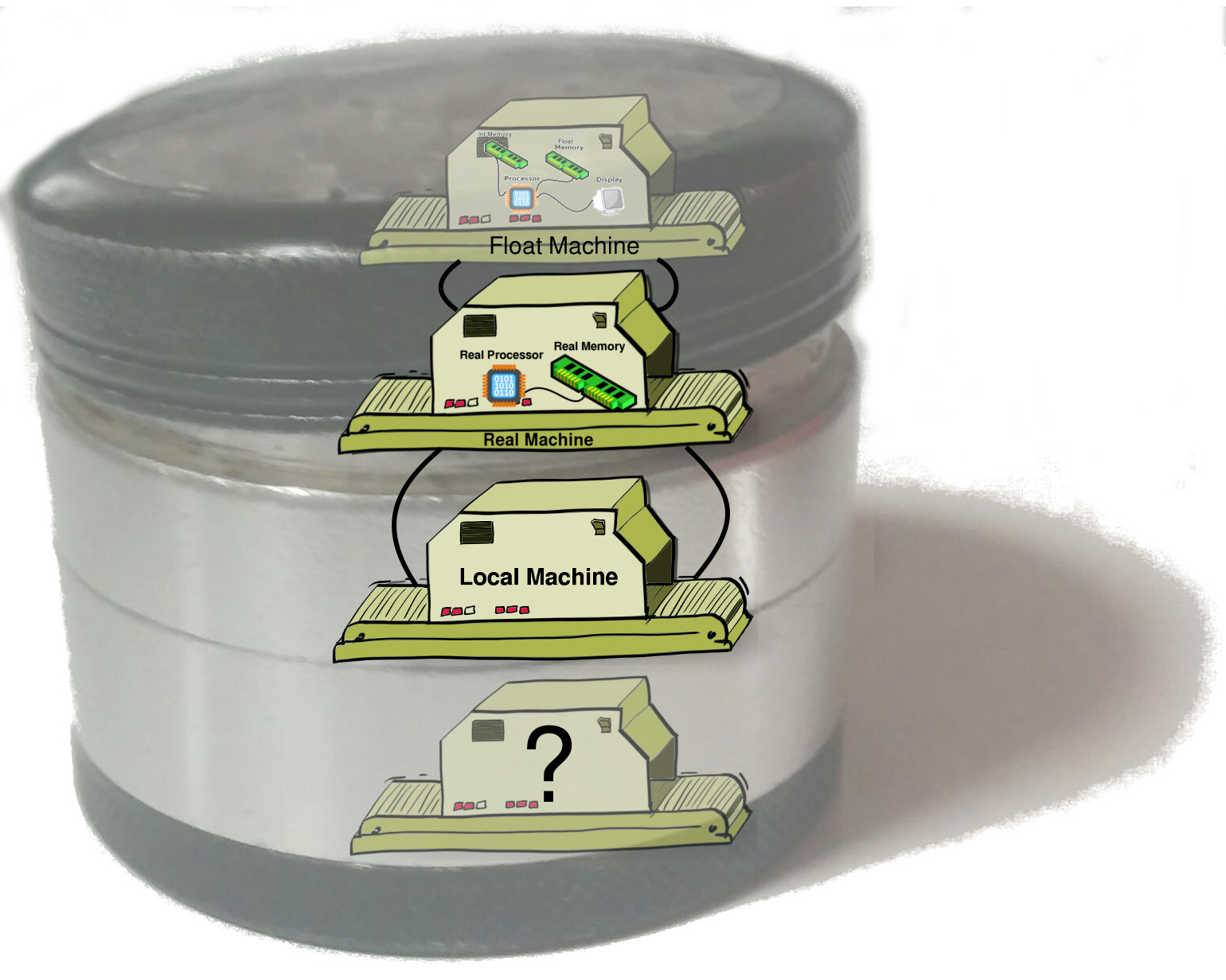
The next machine we’ll add to Herbgrind helps you find the source of error. We’ll call it the “Local” Machine, because it localizes error to a particular place in the program. Now that we have both the real and the float machines, we can watch the “ideal” answer a program should produce, and the actual answer it did produce. By monitoring both of these, the Localizing Machine can determine where error actually arises.

Unfortunately, reporting every place that has error occurs is a little too much, because not all sources of error affect the final result. So, in addition to tracking where error pops up, the Localizing Machine will also track which values in the program are influenced by such error. When the final result is affected by error, we know that it’s bad, and needs to be reported to the user.

For the rest of the post, I’ll try to explain two things:

• How do we detect “local error”? That is, how do we find the place where error first appears?
• How do we track which error affects which values?

Finding Local Error

How do we figure out when error appears? In the last post we introduced the Real Machine, which can track the correct value of the computation, alongside the result that actually gets computed. Tracking the difference between these two executions is useful for figuring out how much error there is in the final answer.

Unfortunately, it’s not quite enough to figure out where error first appears, because once there’s error in one place, that error often makes every answer derived from it also erroneous.

Let’s look at a simple example. Say we want to compute the formula:

Let’s say we’re computing this for \(x = 10^{15}\).

The Real Machine will (correctly) compute this as:

When we watch the Float Machine’s execution at every step, and check it’s error against the correct (rounded) answer, we see this:

It might seem strange that the result of \(x + 1\) isn’t marked as having error. This is because while the correct real number answer is \(1000000000000001\), \(10^{15}\) is the closest floating point number to the correct answer. However, once the subtraction occurs, we get 0, which is NOT the closest floating point number to 1.

If we just told the user about every value that deviates from the correct answer, we would report many locations which aren’t actually at fault for the error, but just a victim of it. By overwhelming the user with candidates to be inspected, we would make it much harder for them to take action to fix the error. So instead of asking the question, at every step, “How far is the result of this operation from the correct result?”, we can ask a slightly different question: “How far would the result of this operation be from the correct result if its inputs were correct?”.

By using the correct versions of the inputs, we make sure not to penalize an operation for the error that happened before it. But, because we still execute the operation itself in floating point precision on floating point inputs (the correct inputs rounded), we still see any error that the operation itself produces.

In the above example, this would look like:

Notice that even though the computation of \((x + 1) - x\) produces the wrong answer, we don’t allow that error to propagate forward because we replace it with the correct answer, from the Real Machine, before computing the next operation. This way, we only report a single location of local error, the subtraction where the error first appears.

The Localizing Machine does exactly this. For each operation instruction in the program, the Localizing Machine pulls the correct arguments from real memory, and rounds them to float. Then, it executes the operation on these rounded correct arguments, and tests to see how far the result is from the correct result computed by the Real Machine. If the locally approxmate answer computed is far from the correct answer, then the current operation has local error.

Now that we know where error is coming from, we need to figure out where it matters, and which sources of error are affecting which outputs.

Tracking the Influence of Error

To figure out what values are “influenced” by error from what operations, Herbgrind uses something called “taint analysis”. It’s a trick that a lot of dynamic analysis tools use, where you attach a “taint” to some values, and propogate that taint through certain operations. In this case, our “taint” will mean “I was influenced by local error x”, where x is the name of a source of local error. Whenever we execute an operation, if any of the arguments are influenced by something, then we say the output is influenced by that thing too.

To make this a little more concrete, let’s look at it in our running example:

Here you can see that the location of error get’s marked with “Location #1”, to indicate that it is affected by the error at the first error location. Since this example only has one source of error, it is called “Location #1”; if there were more sources of error each one would be given a unique name.

Once this label appears, it gets copied to all the values that derive from that location. This way, the final result shows that it was influenced by that location of local error.

That’s basically all there is to the Localizing Machine! It computes the local error at each operation, and marks those that would be significantly inaccurate even if the their inputs were as correct as possible. Then, it propagates those marks through future operations, so that Herbgrind can figure out which sources of error affected the final result.

Now we can add the Localizing Machine to the Float Machine (which runs the programs normally), and the Real Machine (which finds the correct result of the program).

With what we’ve got so far, we can detect erroroneous outputs with the Real Machine, and find the sources of error that influenced them with the Localizing Machine. However, there’s one piece missing, because responsibility for error lies with not just one operation, but a whole sequence of operations. In the next post, we’ll talk about the last machine, which solves this problem.