Herbgrind Part 2: The Real Machine

Welcome back to my series of posts on Herbgrind, a dynamic analysis tool that finds floating point issues in compiled programs. The purpose of this series is to explain how Herbgrind works and the principles behind its design. To do that, we’re starting with a simple hypothetical computer called the “Float Machine”, which is just enough to capture the interesting floating point behavior of a real computer, like the one that’s probably sitting on your desk.

In the last post, we defined the Float Machine. This meant talking about how it executes, and what its programs look like. In this post, I’ll describe how Herbgrind determines how much error is in a Float Machine program.

Analyzing Programs for the Float Machine

In the last post, we introduced the float machine, a simple machine which can run floating point programs in its own language. This language has three instructions: an “operation” instruction which takes some values from memory, runs a floating-point function on them, and puts them back in memory; a “branch” instruction which jumps to a different part of the program if some condition holds; and an “output” instruction which prints a value to the screen.

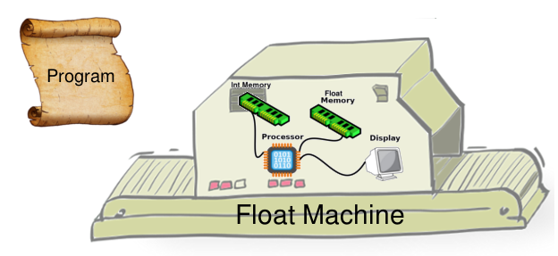
We can think of Herbgrind as just another machine that runs these programs, but runs them slightly differently. The Herbgrind machine includes the Float Machine as part of it, so that it can report information about the actual execution. But it also has some more sub-machines, which execute the program in other ways, and sometimes talk to each other.

The machine we’ll talk about in this post is called the Real machine, because it executes the program in the real numbers. But first, we’ll talk about why we need this machine. In Herbgrind, each machine solves a problem. And the first problem that people face when trying to find the cause of floating point error, is that floating point error is generally silent.

A Primer on Silent Error

Floating point error, unlike other types of bugs in a program, doesn’t generally have a place where it “happens”. Instead it’s something that slowly grows through multiple instructions, so that at any given point it’s not clear how “wrong” the computed answer is.

This may seem counter-intuitive. After all, an answer is either wrong or it isn’t, right? To get a sense of how error can appear without any particular step seeming bad, let’s look at a simple example.

Let’s say you’re computing the formula:

This formula looks reasonable (although a bit redundant) at first. A few simple mathematical transformation can show us that the value of this formula is 1 for any value of \(x\).

However, when the original formula is run in floating point, and given a large value of \(x\), it’ll return 0 instead of 1! For \(x = 10^{16}\), \((x + 1)\) isn’t representable in floating point, so the 1 gets rounded off. This means the entire computation goes like this:

You can see that the error appears in the second line, when the 1 gets rounded off, resulting in the wrong answer in the end.

However, looking at each piece of the computation in isolation, it’s not clear that anything particularly bad is happening. Just looking at the addition which actually causes the error, you would see:

The correct answer is \(10^{16}+1\), but the computation gets \(10^{16}\). But, \(10^{16}\) is actually the closest floating point number to \(10^{16}\), so it’s not actually possible to do this addition any better. And, even if it were possible to do better, relative to \(10^{15}\), this difference is pretty small. Depending on what you do with it afterwards, this amount of error might not matter. For instance, if you were to divide the result by \(10^{16}\), then you would get 10 vs. 10.0000000000000001, which is a negligible amount of error (and once again, not representable any better in 64-bit floating point).

The next step isn’t any more clearly wrong either. After all, 0 is the right answer when subtracting \(10^{16}\) and \(10^{16}\). Because we’ve lost the information on how the orignal answer was slightly wrong, you can’t see at this step that there is now major error.

Calculations like this are why floating point error is generally silent. You wouldn’t want the computer to crash every time it had to round the answer a small amount. But these tiny errors can grow later, and their growth is virtually undetectable

Making The Error Loud

To fix this, we need to create some way to check the answer at every step, and see how far it is getting from the “correct” answer. Since we use floating point to approximate the real numbers, we want to say an answer is “correct” when it’s just like the real number answer. Unfortunately this idea of correctness is a little too strong. Since there are an infinite number of real numbers, and only a finite number of floating point numbers, not every real number can be perfectly represented in the floats. So instead of saying an answer is correct when it’s exactly the real number answer, we’ll say it’s correct if it is the closest floating point number to the real answer.

Put another way, we can say that a floating point program is perfectly correct if the following equation holds:

This says that for every floating point input \(x\), if we convert that number to a real number (\([[x]]_{\mathbb{R}}\)), and then run the program on it as a real number program (\(\texttt{prog}_{\mathbb{R}}\)), and finally round it back to a float (\([[\_]]_{\mathbb{F}}\)), we get the same answer as when we compute it normally using floats (\(\texttt{prog}_{\mathbb{F}}\)). This is the best accuracy we could possibly get from a floating point program.

This definition might not seem like it’s giving us anything extra, but we’ll see that by applying it to the whole program, instead of just each operation, we can catch the error which would otherwise be silent. To apply this definition to the whole program, though, we’ll need to have someway to compute what the program should have been, in the real numbers. This is the first task of the Real Machine.

The Real Machine is a lot like the Float Machine from the last post, except it does everything in the Reals. It uses the same program as the float machine, but it has a “Real” processor which can do real number calculations, and “Real” memory for storing these real numbers.

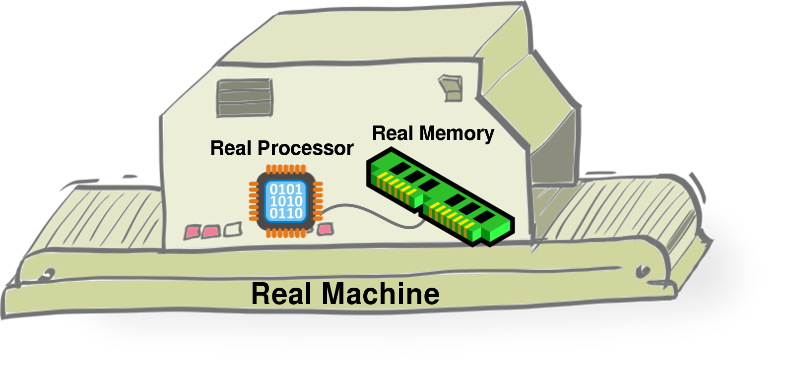
Since the Real Machine only checks the accuracy of the float machine, it doesn’t need its own output. And since it only cares about floating point calculations, it doesn’t need its own int memory (memory that holds non-float values). But to keep track of where it is in the program, and check the error of the float machine, it depends on being connected to the float machine.

With the Real machine, we can finally identify whole program error. But we still need a way to determine whether the error is large or small. For this, we have to quantify the error that appears.

Quantifying Error

Since programs often don’t compute the “correct” answer, it’s useful to know how far the result is from the right answer. If it’s not exactly right, but very close, then in a lot of situations we don’t care. However, even for simple programs, sometimes the answer computed is very far from the right answer. We’re going to call the distance between the computed answer and the right answer the “floating point error” of the program.

This definition leaves two things open. One is that we haven’t defined what it means to be the distance between two floating point numbers, in this equation represented by the function \(\varepsilon\). And this definition is for how much error a program has on a particular input; what about the program as a whole? For both of these questions, there isn’t one right answer. But we can pick some that tend to be pretty useful in practice.

The Error Between Two Numbers

First, let’s think about how to measure the distance between two floating point numbers. When we’re measuring the distance between two real numbers, it’s common to use either absolute error, or relative error. Absolute error is just the actual difference between the numbers:

While relative error is the difference as a fraction of the right answer:

Absolute error is nice because it’s a relatively simple, intuitive notion. However, its problem is that it doesn’t capture the notion that error means different things on different scales. If a program is supposed to return 1,000,000, and it instead returns 1,000,001, we don’t usually think of that as very much error. But if it is supposed to return 0, and it returns 1, that’s pretty bad. With absolute error, both of these differences are treated the same.

Relative error helps fix this problem by scaling the error according to the right answer. However, it has its own problems. Since it divides by the correct answer, what do you do when the correct answer is zero? And how do you account for the fact that floating point numbers aren’t spaced exactly exponentially, so numbers of different sizes will tend to have more or less relative error?

To address both these issues, Herbgrind borrows a tool from StokeFP and Herbie. Both of these program transformation tools measure error in something called Units in the Last Place, or ULPs. Essentially, this measures how many floating point values there are between the correct answer, and the answer that you got. For instance, if those two numbers are right next to each other (there are no floating point values in between), but not the same, the error is 1 ULP. If the answers are as far as they can possibly be from each other, the error is \(2^{64} - 1\) ULPs.

You might notice that there’s a 64 in that number, just like the number of bits used in your computer to represent (double-precision) floats. This isn’t just a coincidence: if you take the \(\log_2\) of the number of ulps, you get something like the number of bits different between two floating point numbers. So we can say that two values on the opposite ends of the number line have “64 bits” of error, and two values that are right next to each other have “1 bit” of error.

Aggregating Whole Program Error

Now that we know how to measure the error on a particular input using our \(\varepsilon\) function, we want to know how to give an error score to the whole program, not just on a particular input.

To do this, we’re going to measure two things: the error in the worst case, called “max error”, and the error in general, called “average error”. In some applications, it’s super important that the answer never be very wrong. For those, it’s useful to pay attention to the max error. In other applications, you just want to have most of your answers be correct. We found while working on Herbie that floating point error tends to be either really big or really small, so average error generally measures how many inputs are really bad.

Phew, that’s a lot of information. Okay, now we know:

• What floating point error is
• How to measure it for a particular input
• How to grade a program on its floating point error

With just this Real Machine, Herbgrind can detect error in floating point programs, and tell you how bad it is. But Herbgrind’s mission isn’t over. Knowing how bad your floating point error is isn’t enough to help you fix it: you have to know where it comes from. The next posts will define some more machines that Herbgrind uses to find the cause of floating point error in a program.