Herbgrind Part 1: The Float Machine
In the previous post here, I wrote about how I got started working on a new floating point tool, Herbgrind. Herbgrind is a program analysis tool that finds numerical issues. To understand how Herbgrind gets there, I want to start from the basics, to introduce the concepts in an easy-to-understand context.
This post is the first in a series where we build up Herbgrind, starting from an abstract floating point program and analysis, and eventually getting to the systems which allow Herbgrind to find numerical errors. In this post we’ll define a simple machine which can do floating point calculation, and go over a simple example program. This is the machine which we’ll use to define Herbgrind’s analysis in future posts.
So let’s get to it.
What is a floating point program?
Well, it’s a program, so it runs on some sort of machine. And it uses floating point, so that machine must have some way of doing floating point calculations. Floating point is a number representation that computers use to approximate math with real numbers. It’s a bit like “scientific notation” you might have read about in high school; for a bit more background on how it works, check out my post on Kahan summation here. Real-world machines like the one you’re reading this on are big and complicated, so to start, we’ll talk about a much more basic machine. We call it a “Float Machine”.
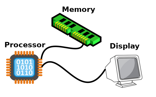
The Float Machine has three parts: a processor, some memory, and a display. This will let us compute on floats, store them somewhere and load them later, and produce output. We’ll ignore input from the user, and assume that all “inputs” are encoded in the program.
Wait, what’s a program? Okay, a program is a big list of instructions, where the instructions are numbered starting at 1. Instructions tell the processor to do something with the data in memory, and maybe write something to the display. The machine will keep track of a number to tell us which instruction we’re currently executing, called the PC, for program counter. There are going to be three types of instructions: operations on values, conditional branches, and output statements. It turns out, with just these three things (well, really just the first two, if you’re willing to read the memory afterwards), we can write any computation that runs on any computer.
Let’s make this a little more concrete.
Operations
We’ll define an “operation” instruction as having three parts: a function (like +, -, or sine1), information about where the inputs come from, and information about where the output goes. Since memory is just a big array of values, we’re going to use numbers to represent locations in memory. For instance, you might have an operation like:
\[\texttt{memory}[25] \gets \texttt{memory}[42] + \texttt{memory}[0]\]or
\[\texttt{memory}[45] \gets \sin(\texttt{memory}[30])\]In a C-like language, you might write these as:
memory[25] = memory[42] + memory[0]
memory[45] = sin(memory[30])
Each of these instructions has a function (\(+\) and \(\sin\)), memory locations where the inputs come from (\(\texttt{memory}[42]\), \(\texttt{memory}[0]\), and \(\texttt{memory}[30]\)), and memory locations where the output goes (\(\texttt{memory}[25]\) and \(\texttt{memory}[45]\).
Since our language doesn’t include constants explicitly, we’ll sometimes have operations which take no arguments, and produce a constant result, like:
\[\texttt{memory}[57] \gets Const4()\]You can think of this as:
\[\texttt{memory}[57] \gets 4\]Branches
A branch instruction is a little more complex, because it’s going to change the control flow of our programs. Every programming language has something like this, in a C-like language it might look like this:
if (cond(memory)) { // cond is a predicate
    // do something
} else {
    // do something else
}
In this example, we have some function cond which returns “true” or “false”
based on the state of the memory. Functions that return true or false
are generally called predicates.
For our float machine, we’re going to make branches even simpler. First of all, we’ll specify which cells in memory the predicate can use. Next, instead of marking blocks of code as true or false, we’re going to specify an alternate PC to jump to. That way, when the predicate returns true, we will set our PC to the alternate PC specified by that branch. Otherwise, we’ll just increase it by one like normal.
For example, the instruction:
\[\texttt{if}\ (\text{LESS}(\texttt{memory}[57],\ \texttt{memory}[28]))\ \texttt{goto 45}\]skips to \(\texttt{instruction[45]}\) if the value at location 57 is less than the value at location 28, and just goes to the next instruction otherwise.
Finally…
Output
The last type of instruction is an output instruction, like:
\[\texttt{output}\ \texttt{memory}[64]\]This takes a location in memory, and prints the value there to screen. A program can output as many times as it wants. When the user looks at the program’s behavior, all they see is the outputs that printed. An output instruction doesn’t affect the state of memory, or the PC, it just prints to the screen.
A (Relatively) Simple Example
Let’s look at an example program. Say we want to get the absolute value of the \(\sin\) of 7. This doesn’t really mean much, math-wise, since \(\sin\) is a function that gets applied to angles measured in radians (180 degrees = \(\pi\) radians), but it’s a nice example. This is a program that computes what we want2:
| 1 | \(\texttt{memory}[1] \gets Const7()\) |
| 2 | \(\texttt{memory}[2] \gets Const0()\) |
| 3 | \(\texttt{memory}[3] \gets \sin(\texttt{memory}[1])\) |
| 4 | \(\texttt{if}\ (\text{LESS}(\texttt{memory}[2],\ \texttt{memory}[3]))\ \texttt{goto 6}\) |
| 5 | \(\texttt{memory}[3] \gets \texttt{negate}(\texttt{memory}[3])\) |
| 6 | \(\texttt{output}\ \texttt{memory}[3]\) |
| 7 | \(\texttt{if}\ (ConstTRUE())\ \texttt{goto -1}\) |
Let’s walk through this a line at a time:
\(\texttt{instruction[1]}\) is an operation which puts the value 7 into \(\texttt{memory[1]}\). Since operations can take any number of arguments, we’re allowed to define the operation \(Const7\) to take zero arguments, and always produce 7. \(\texttt{instruction[2]}\) puts the value 0 into \(\texttt{memory[2]}\).
\(\texttt{instruction[3]}\) is our first real operation:
| 3 | \(\texttt{memory}[3] \gets \sin(\texttt{memory}[1])\) |
This line takes the value at \(\texttt{memory[1]}\) (\(7\)), runs it through the \(\sin\) function, and puts the result in \(\texttt{memory[3]}\). After all three of these instructions are run, memory looks like this:
| 1 | 7 |
| 2 | 0 |
| 3 | 0.6569… |
| … | … |
Now that we’ve got \(\sin(7)\), we next need to find its absolute value, and for that we’ll need a branch. If the value is less than zero, then we’ll need to negate it.
In this example the number \(7\) is fixed, but in general we can imagine these programs as having a bunch of code written once, with some special memory locations for the inputs. Then, whenever someone wants to run them, they’ll put their inputs in those memory locations, and let it run. In that case, when you’re writing the code, you won’t actually know what the inputs are.
The next instruction:
| 4 | \(\texttt{if}\ (\text{LESS}(\texttt{memory}[2],\ \texttt{memory}[3]))\ \texttt{goto 6}\) |
is actually going to do the branch. Here, we run the LESS predicate over the value at \(\texttt{memory[2]}\) and the value at \(\texttt{memory[3]}\). \(\texttt{memory[2]}\) holds 0, since we put it there at the beginning of the program, and \(\texttt{memory[3]}\) holds \(\sin(7)\). LESS will return true if \(0 < \sin(7)\), and false otherwise. In this case, since \(\sin(7)\) is positive, it’ll be true. That means that instead of just going to the next instruction after this one, we’ll “jump” over to instruction 6.
If \(\sin(7)\) were negative, we wouldn’t have jumped, and instruction five would have negated \(\sin(7)\), making it positive.
Since we did jump, we’re now at \(\texttt{instruction[6]}\):
| 6 | \(\texttt{output}\ \texttt{memory}[3]\) |
which prints out the value we’ve computed, \(|\sin(7)|\). This provides the “answer” of the program to the user.
Finally, we’re going to run \(\texttt{instruction[7]}\) to terminate the program.
| 7 | \(\texttt{if}\ (ConstTRUE())\ \texttt{goto -1}\) |
This is another conditional jump, but the predicate always returns true. Why would we want that? Well, it allows us to jump to the special instruction \(\texttt{instruction[-1]}\) unconditionally. When the float machine gets to \(\texttt{instruction[-1]}\) it stops.
So that’s a simple program. The programs we care about are going to be much more complex, but they all can be modeled using these simple pieces. That way, we only have to worry about what to do with each piece, and we can handle huge programs that do complicated things.
Upgrading the Float Machine
The machine we’ve constructed so far can do any floating point calculation you can dream up. It’ll be a useful base for defining what Herbgrind does to help programmers find dubious floating point code.
However, before we do that, let’s make one more modification to the machine. In a real computer, not all calculation is done in floating point. There are also more integer-like types, that do almost everything in your computer. Even though you can technically emulate these with floats, we’ll add integers to the float machine, so that we can talk about the distinction between code that deals with floating point, and code that doesn’t.
Real-world machines put integers and floats in the same memory bank, but
this part isn’t really important for Herbgrind, so to simplify things
we’ll give an extra type of memory to our computer: int
memory.
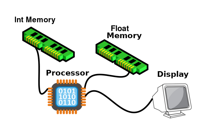
int memory is indexed just like float memory, but contains integers
as values instead of floating point numbers. Since both memories have
slots for every address, we need to have a way to tell if a program
instruction is talking about int memory or float memory. We’ll do this
by creating an int version of every instruction: int operations
take integer arguments and produce an integer, int branches take
int predicates which operate on integers, and int output prints
out an integer.
We’ll also add conversion operations, both float-to-int, which takes
floating point arguments and produces an integer, and int-to-float,
which takes integer arguments and produces a float.
And that’s it! That’s the Float Machine. For now that’s not going to be very useful, unless you particularly like thinking of novel ways of building a computer, but in the next post, I’ll talk about what Herbgrind does to this machine to detect and report its error.
-
The sine function is a trigonometric function, which can’t be defined through finite arithmetic formulas. It returns values between -1 and 1, and repeats every 2\(\pi\). For the purposes of this post, you don’t need to know exactly what it does. Sine is often written “sin” in code and math. ↩
-
I’m using green for programs, and blue for memory in this post. ↩