Herbgrind Part 6: Let's Get Real

Welcome back to my series of posts on Herbgrind, a dynamic analysis tool that finds floating point issues in compiled programs. The purpose of this series is to explain how Herbgrind works and the principles behind its design. To do that, we started with a simple hypothetical computer called the “Float Machine”, which is just enough to capture the interesting floating point behavior of a real computer, like the one that’s probably sitting on your desk. Now, we’re bringing Herbgrind’s analysis to the real world, making it computable and fast.

If you missed the previous posts in this series, you might find this one a bit confusing, so I suggest you go back and read it from the beginning. If that’s too much reading, the post right before this one has a short summary of the lead up, and introduces the Valgrind framework which this post builds on. In this post, I’m going to assume you know what I mean when I talk about “the Real Machine”, or “thread state”.

Let’s get started.

Bringing The “Real Processor” Into The Real World.

Herbgrind is a tool designed to help users deal with floating-point code, which tries to approximate the real numbers. Of course, this wouldn’t be a problem if we could just compute with the real numbers in the first place, but it’s not possible to actually represent the real numbers on a computer. There’s a way to get something close enough that it’s basically the real numbers for all intents and purposes, called the computable reals, but they tend to be very slow. So we’re stuck with the floating point numbers for many applications, and the pitfalls that come with using them.

Hopefully, Herbgrind can help users navigate those pitfalls, by pointing out where error is occuring, and what is causing it. But to figure out where the answers your program is producing are “incorrect”, we need to know what the “correct” answer is. And to do that, we need to compute with the real numbers. See the problem here?

In the abstract version of Herbgrind, given in parts 1-4 of this series, we didn’t worry about how we’d compute the real number answer, because we were working in the abstract. But now that we’re trying to bring Herbgrind to a real computer, we need to figure it out.

The solution comes from a great library called GNU MPFR, or sometimes just MPFR for short. MPFR stands for Multi-Precision Floating-point Reliably, because it allows you to do floating point calculations with any number of bits, instead of just 64- or 32-bit floats¹.

MPFR numbers still aren’t real numbers, since they still only have a limited number of bits. But adding more bits to your representation generally means you get closer to the real numbers². So, if your 64-bit answer and your 1000-bit answer disagree, your 64-bit answer is definitely not the same as the real number answer. Another way to think of this is that if you measure the error of the 64-bit answer with respect to the 1000-bit answer, you’ll get a lower bound on the error of your 64-bit answer with respect to the real numbers.

You might be thinking, “if MPFR numbers are so great, why not just use them for all of our floating-point math and be done with it?”. And for some applications, that’s a great solution. Unfortunately, operations on MPFR numbers can be hundreds to thousands of times slower than their hardware floating-point counterparts. So for many of the applications which we use floating-point for, they are just too slow. In Herbgrind, however, we’re okay with being slower than a regular program, because we’re only trying to find the floating point errors, not monitor the program every time you run it.

With MPFR in our toolbox, we can implement the “Real processor” outlined in the earlier post about the Real Machine. But there’s still another part to the Real Machine, “Real memory”, which is trickier than it at first appears.

Memory For Reals

In the idealized Float Machine, floating-point memory was just a big list of numbers. Every operation in the program referred to locations in this list to take it’s arguments from, and a location to put the result in. When we added the idealized Real Machine into the mix, it had a parallel list of real numbers, and “mirrored” all of the operations on those. Now that we’re working on the VEX machine though, things get more complicated.

Mixed-Type Memory

In the Float Machine there were two memory banks, one for integers, and one for floating-point numbers. In the VEX machine there is no such distinciton: any location could hold either³. The simplest solution to this issue is to treat every location in memory as a float, given a shadow value at the beginning of the program. Unfortunately, this would mean creating a shadow value for every location in memory, thread state, and temporaries, which would take far too much space!

Instead, we’ll take a lazy approach. At the beginning of the program, we’ll assume each value is a non-float. Then, whenever we run a floating point operation, we’ll mark both of it’s inputs as floats, give them shadow values based on their current value, and execute the operation producing a shadow result. This lazy approach is pretty efficient, only storing the shadows that we might need.

This approach leaves a lot of program statments untracked. Before its first floating point operation, a value might be moved around, packed into data structures and unpacked, and have its bits flipped for various reasons. But none of these statements can introduce floating point error, since they don’t correspond to any real number operation. Even if a value came from some other part of the program and had arbitrary transformations done on them, we wouldn’t know how to interpret those operations as real number transformations. The first time we have any possible error to track is exactly when we make the shadow value for the first time: at the first floating point operation.

It has one subtlety though, and that comes with how it interacts with the many ways of representing floats. You see, the VEX machine doesn’t have a single type of floating-point number, it has two; just like an x86 processor, or any other modern processor for that matter, VEX includes both 32- and 64-bit floats[^no-80-bit]. It also happens to represent values which are packed into an array of up to 256 bits. VEX of course contains instructions for converting between these formats, like turning a 32-bit float into a 64-bit one, or pulling a 32-bit float out of the first quarter of a 128-bit array. So what do we do when these kinds of operations are run on something that we have not yet determined is a float?

[^no-80-bit] 32-bit processors using x87 also include 80-bit floats, bur they can cause a myriad of problems. Herbgrind has been developed for 64-bit processors, and only really supports SSE and it’s sucessors, which became the standard in the early 2000’s (first released in 1999). As a result, we don’t really deal with 80-bit floats.

Well, it’d be safe to treat them like a floating point operation, and add a shadow value to them. But we don’t really have to do that, do we? Since these operations can’t have any error, it’s totally safe to ignore them if they’re run on bytes that aren’t shadowed yet. But if the bytes are already shadowed, we’ll need to do the proper transformation on the shadow; just transforming the bytes means we might lose information about the exact value. So for these conversions, we’ll treat them like floating-point operations if they are running on something we already know is a floating-point number, and we’ll treat them like integer operations otherwise.

Expensive Shadows

Even when we’re only shadowing values which are actually floats, shadow values can be really memory intensive! For each 32- or 64-bit float, just the real number shadow takes upwards of a thousand bits, not to mention the extra information we’ll be tacking on later!

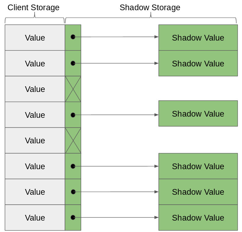
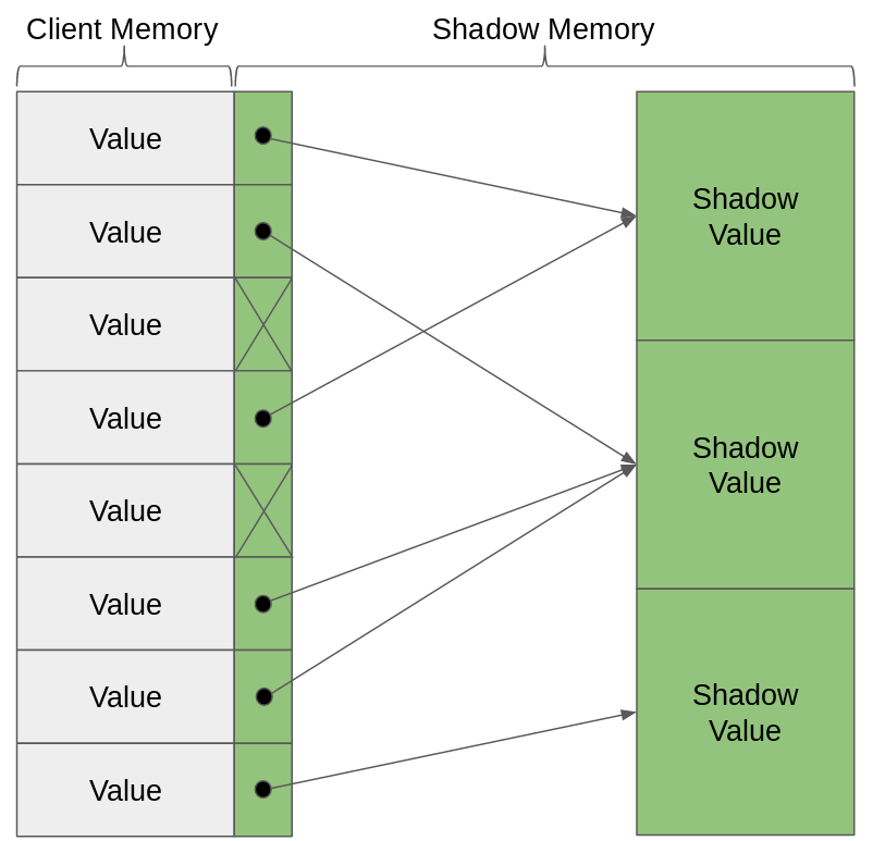
Luckily, we can exploit some redundancy in the program to get that cost down. You see, most of the floating point values you’ll find in a program’s memory aren’t unique. Lots of them are just copies of one another, created because multiple parts of the program need to use the same value, or simply a by-product of copying the value to move it around, and not deleting the old copy. Since values are often identical, we don’t always need to shadow them with separate shadow values. Instead, we can use the same shadow value for every copy of the same value.

Unfortunately, just because two values have the same literal bytes doesn’t mean we can treat them like copies; they could have different exact values, but just be rounded to the same thing. But when we see a copy instruction, instead of creating another shadow value for the copy, we can just add a new reference to the old shadow.

In many programming languages, when we create multiple references to the same object, the language will automatically manage the memory for that object, and figure out how to free the object when the references are gone. But when we’re writing our analysis inside valgrind, we’re working outside the structures of these high level languages. Herbgrind (like most Valgrind tools) is written in C, which is low-level as it is, but the code which runs at runtime (after the program has been instrumented) is even lower-level in a sense, and extremely performance sensitive. So we won’t get anyone helping us with managing the memory of our shared shadow values, we have to do it ourselves.

The simplest approach to memory management is just to make copies of everything, and share nothing. This way, every piece of the code knows it’s the only one handling its data, and can free it when it’s done. But we already know that’s too expensive for the shadow values in Herbgrind.

The easiest version of memory management from a user perspective is called garbage collection. This means we keep track of all of our most basic references in some sort of table, and then every once in a while stop the program, trace the references to figure out which objects can be freed, and free them. This is the approach that many modern high-level languages, like Java, Python, Lisp, or OCaml, use. Unfortunately this is too time-consuming for Herbgrind, since it means stopping the program and doing complex analysis, in an environment where every instruction counts.

Somewhere in the middle is an approach called reference counting. In reference counting, each object that you want to share has a counter, called a reference count. When it’s first created, and only one piece of code has access to it, it’s reference count is one. Whenever a new piece of code or data gets a reference to that object, we increase it’s reference count. When code or data is done with the reference, and deletes it, it does two things. First, it decreases the reference count. Then, if the reference count is zero, it frees the object.

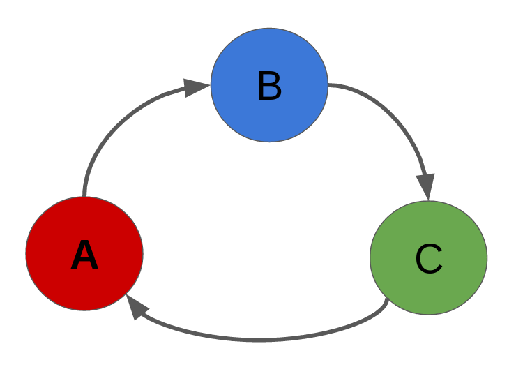
There are two downsides to this approach. First, it doesn’t deal well with cyclic data structures. If object A has a reference to object B, and object B has a reference to object C, and object C has a reference to object A, they might never be freed! Of course, if someone else has a reference to one of these objects, they shouldn’t be freed, but even when everyone else has divested themselves, each object still has one reference to it. To make sure this doesn’t happen, code using reference counting has to be very careful about what kinds of data structures it creates[^herbgrind-cycles].

[^herbgrind-cycles] For the real number shadows, Herbgrind doesn’t generally have to worry about cycles. But once we start dealing with symbolic expression trees, it’s pretty common to have objects which reference each other.

Which brings us to the second downside of reference counting, that it’s heavily error-prone. With no language support, it’s easy to make a mistake, and either count too many references (never freeing the object), or too few (freeing it too early, and potentially trying to use it after).

Reference counting has a big upside in performance though, because it allows us to share objects, with basically no extra runtime computation. In Herbgrind’s case, this makes it the right tradeoff, so it’s what we use.

Multiple Types of Storage

In addition to storage in the VEX machine holding both integers and floating point numbers, and the workarounds needed to keep memory usage down, we also have to deal with the fact that there are now three types of storage where floating point numbers can exist, not just one. With that comes new program statements for moving values around between storage types, as well as some subtleties of the types themselves.

Let’s start with the temporaries, since in many respects they are the simplest. Temporaries in VEX are an infinite list of storage locations, where each location can hold a float, a double, or a few floats or doubles put together. Processors like the x86 family often have instructions that can manipulate several floating point numbers at once. Instead of just taking two floating point numbers and adding them, they can take two blocks containing two double-precision numbers each, and multiply them in parallel. In VEX, this translates into a special mulitply instruction on two temporaries, each of which holds two double-precision values.

These multiple-value temporaries present the first challenge with shadowing temporaries. While we normally only need one shadow value per storage location, in the case of a temporary that holds multiple floating point values, we’ll need multiple shadow values. To handle this, Herbgrind includes a notion of shadow temporary. A shadow temporary is a structure that holds one or more shadow values. It’s not always clear from the size of a temporary how many values are in it: a 128-bit temporary could hold two doubles, or four singles. So we give each shadow temporary a runtime type (as well as a static type, when possible), which indicates how many values it’s shadowing, so there’s no confusion.

We’re going to need some way to keep track of what shadow temporaries coorespond to what temporaries in our VEX program. Each temporary in VEX has a number that represents it, and that the program uses to refer to it (t1, t2, t3, etc). So to keep track of their shadows, we’ll create a similarly numbered list of shadow temporaries. Since we’re not going to shadow all the temporaries, some of these slots are empty (a NULL pointer instead of a pointer to a shadow temporary). But we still have a problem: there are (in theory) an infinite set of temporaries! We can’t hold on to an infinite set of pointers, even if most of them are NULL. So when we first look at each code block to start instrumenting it, we’ll figure out how many temporaries are actually used in practice, and only create a list that big. Just to be safe, we’ll also add a global limit to how many temporaries we’re willing to shadow, so things don’t get too crazy.

After the temporaries are shadowed, the next type of VEX storage that we’ll have to shadow is thread state. Thread state represents the registers and cpu flags of the underlying program. But at the VEX level, it doesn’t look like a bunch of named registers, it looks like an array of bytes. For any register on the processor, there’s a location in this array that cooresponds to it. But instead of this byte array having slots for each value, it’s completely unstructured; it’s just bytes. A single floating-point value can take up four or eight bytes, and you can’t usually count on things being aligned in a nice way.

To handle this, we’ll pretend that each floating-point value can take up a single byte. Then, we’ll shadow the bytes much like we shadowed temporaries, with a parallel list where each shadow aligns with the thing it’s shadowing in the original list. But when we store a floating point value in a location in thread state, we’ll store it’s shadow in the first byte of that location in the shadow thread state, and then mark some of the bytes after as “non-float”. For instance, if we’re storing a 64-bit float in thread state at byte 240, we’ll store it’s shadow in shadow thread state at byte 240, and then set bytes 241, 242, 243, 244, 245, 246, and 247 to “non-float”.

The last type of storage is memory. Memory is a list of bytes like thread state, so we’ll use the same trick we just described to shadow it. But unlike thread state, memory is huge. And unlike the temporaries, we’re not always storing values right at the beginning of memory (in fact, we rarely are), so we can’t just pick a reasonable prefix of memory to shadow. Instead, values can be stored all around, sometimes seperated from each other by gigabytes of “dead” space.

So instead of using a big array to store our values, we use a hash table. For those who aren’t familiar, a hash table is a mapping from keys to values, with constant lookup time, and using much less storage than the number of possible keys. In the case of shadow memory, our keys are memory addresses, and our values are shadow values. With the magic of hash functions, we can allow storing shadow values at any memory address, without having to use as much space as all of memory when we’re not storing things in all of memory.

Now that we’ve figured out how to shadow all these types of memory, the rest is reasonably straightforward (well, until you try to actually implement it…). When we see an instruction in the original program which moves a value from memory to thread state, for instance, or from a temporary to memory, we will add an instruction which moves from the shadow temporary which cooresponds to the source location, to the shadow destination. When we see a floating point instruction in the original program which is doing some sort of mathematical operation, we’ll create shadow values for the arguments if they don’t exist, and put the shadow result in the shadow destination. With just these two parts (a way to create and manipulate shadow values, and a way to move them around), we can track the entire execution of the program. When it’s finally done, wherever it puts the result, we’ll find an exact result in the cooresponding shadow temporary.

That’s pretty much it for the Real Machine! With these parts, we can get the (almost) exactly correct result, and we can compare it to the computed result to figure out how much error there is.